This is a continuation of a discussion about quantization and analog-to-digital converters. In that discussion, the normalized quantization step through an N-bit ADC was denoted q, where q = 1/2N. The ADC encoder transfer function yielded a quantization error range over the interval [-q/2,+q/2].
Quantization is a highly nonlinear process. Denoting the input and output of a quantizer as u[n] and uq[n], respectively, the error from quantization uq[n]-u[n] can be re-arranged to yield the additive noise model of quantization error: uq[n]=u[n]+e, where e is the quantization error.
The figure below shows the quantization error for a full-scale sine wave over a single period. Also shown is the quantization error for a full-scale sawtooth ramp signal.

Although the quantization error from the sinusoid is signal-dependent and nonlinear, the commonly used additive noise model assumes a stochastic process in order to simplify the analysis. In particular, the error is treated as an independent and identically distributed (i.i.d.) random variable.
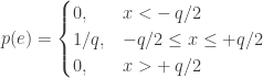
If the quantization error is modeled as a random variable with a uniform distribution, the probability density function is given by:
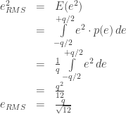
The root mean-square (RMS) quantization error with such a distribution can thus be derived:
The RMS value of a full-scale sinusoid whose peak-to-peak swing has been normalized to unity is given by:

The signal-to-quantization-noise ratio (SQNR) through the ADC can then be computed and expressed in decibels (dB) as:

Substituting q=1/2N gives:

This is the well-known equation for SNR or dynamic range through an N-bit ADC using the additive noise model of quantization error, and in the absence of all other noise sources like thermal noise in the analog circuitry, dither and sampling jitter. Note that no over-sampling is assumed here.
This analysis assumes that quantization errors are uniformly distributed over the quantization interval. In reality, the errors are not uniformly distributed for a sinusoidal input. For example, referring back to the time-domain quantization error from a sinusoid and a sawtooth ramp shown in the figure above, the respective error distributions are shown in the figure below.

The quantization error of the sawtooth wave appears to be uniformly distributed, but that of the sinusoid is clearly not. This is due to the signal-dependence of the sinusoid’s quantization error. Since the sawtooth actually produces uniformly distributed quantization errors, it is instructive to compute the SQNR from quantizing such a signal.
The RMS value of a full-scale sawtooth whose peak-to-peak swing has been normalized to unity is given by:

Using the RMS quantization error derived above for a uniformly distributed quantization error, the SQNR of a sawtooth wave applied to an ADC can be expressed as:

In general, the computed SQNR depends on the signal source and the model used for the quantization error. For sinusoidal inputs, the approximation of uniformly distributed quantization error improves as the ADC precision increases.
The figure below compares the error distribution of the sawtooth with that of four ADC resolutions (3 bits, 6 bits, 9 bits, and 12 bits). Clearly, the distribution approaches the quantization model of a sawtooth as the ADC resolution is increased.

Modeling the SQNR as 6dB per bit of ADC precision is a good approximation, especially as the ADC precision asymptotically increases. For many signal processing applications, the usefulness of approximating the quantization error as an i.i.d. noise source, far exceeds the inaccuracy of the model.
Copyright © 2008 – 2012 Waqas Akram. All Rights Reserved.
Read Full Post »


